You Only Need Minimal RLVR Training: Extrapolating LLMs via Rank-1 Trajectories
Zhepei Wei†, Xinyu Zhu†, Wei-Lin Chen†, Chengsong Huang‡, Jiaxin Huang‡, Yu Meng†
†University of Virginia ‡Washington University in St. Louis
📚 Paper: https://arxiv.org/abs/2605.21468
💻 Code: https://github.com/weizhepei/RELEX
🤗 Checkpoints: https://huggingface.co/relex-rlvr
We find that RLVR weight trajectories are extremely low-rank and highly predictable: (1) the majority of RLVR gains are captured by a rank-1 approximation of the parameter deltas, and (2) the magnitude of this rank-1 projection evolves near-linearly with training steps.
To exploit this structure, we propose RELEX (REinforcement Learning EXtrapolation), which first estimates the rank-1 subspace from a short observation window of RLVR training and then predicts future checkpoints via linear regression, with no learned model required.
This simple method shows promising potentials — using only 15–20% of RLVR training as observed prefix, RELEX matches or even surpasses full RLVR on both in-domain and out-of-domain evaluations across Qwen2.5-Math-1.5B, Qwen3-4B-Base, and Qwen3-8B-Base.
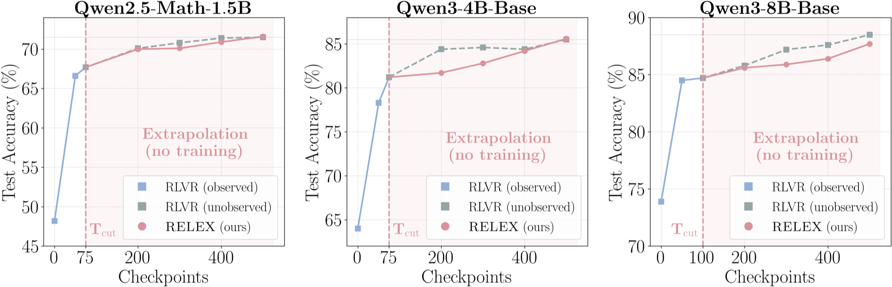
Figure 1. RELEX produces checkpoints that match full RLVR performance based only on early training dynamics, without further training. RELEX first estimates the rank-1 update subspace from the observed RLVR prefix (up to \(T_{cut}\)), then extrapolates future checkpoints at no training cost, matching or exceeding the RLVR checkpoints on the MATH test set across three models.
Motivation
RLVR is powerful but expensive — a typical training run takes massive optimization steps and days of GPU time, even for moderately sized models. This raises a natural question: can we predict where RLVR training is heading from its early dynamics? If weight updates follow a structured, predictable pattern, we could extrapolate future checkpoints from a short prefix of training, potentially achieving the same level of performance as the fully trained model while saving most of the compute.
We start with two concrete questions:
- What to model — what weight-space structure does RLVR induce? Do RLVR gains require modeling parameter changes in full parameter space, or can the majority of gains be captured in a low-dimensional subspace approximation?
- How to model — are these changes predictable via simple function fitting? If the subspace is low-rank, can we describe its dynamics with something as lightweight as linear regression, or do we need a learned predictor?
The following two findings across three backbone models directly answer these questions.
Finding 1: RLVR weight updates are extremely low-rank
We train three models (i.e., Qwen2.5-Math-1.5B, Qwen3-4B-Base, Qwen3-8B-Base) with GRPO for 500 steps on MATH, saving checkpoints throughout training. For each checkpoint at step \(t,\) we compute the weight delta \(\Delta θ_t = θ_t − θ_0,\) and then perform SVD across the delta trajectory to get low-rank approximations of \(\Delta \theta_t,\) which are used to reconstruct/approximate model weights at each step. The result is striking: a simple rank-1 approximation closely recovers the RLVR performance across training steps, as demonstrated in Figure 2.
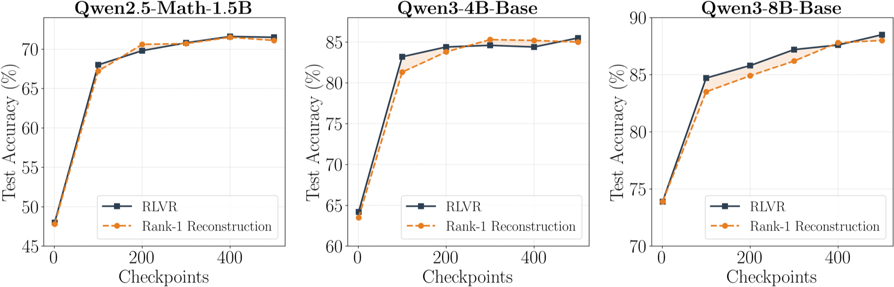
Figure 2. Rank-1 SVD reconstruction closely recovers RLVR checkpoints across models. The rank-1 reconstructed checkpoints preserve most downstream performance on MATH, suggesting that a single dominant direction captures the task-relevant component of RLVR updates.
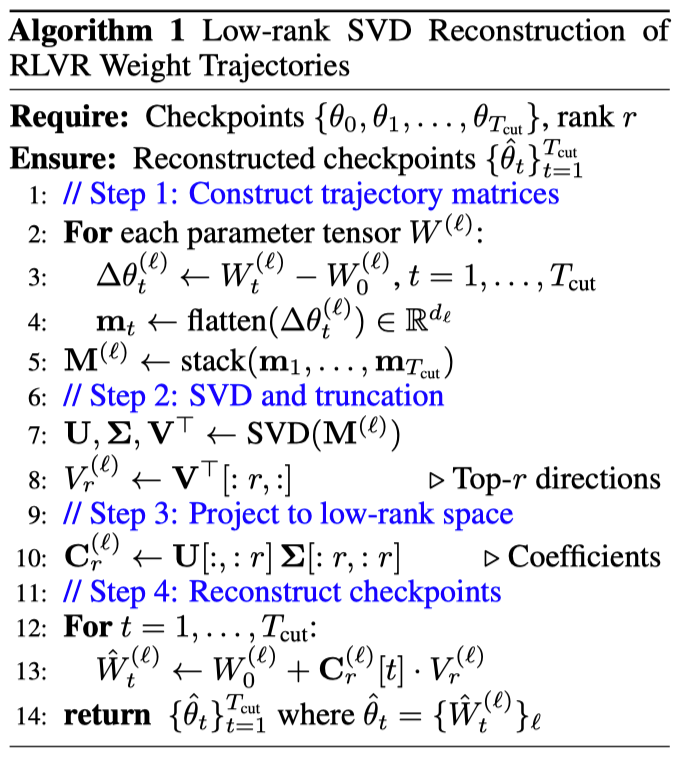
Algorithm 1: Low-Rank SVD Reconstruction of RLVR Weight Trajectories
Finding 2: SVD rank-1 coefficients evolve linearly
With rank-1 projection, the evolution of RLVR-induced update of each weight tensor \(\Delta\theta_t ^{(\ell)}\) at step \(t\) reduces to a scalar time series \(\mathbf{c_t}^{(\ell)},\) which is the projection of deltas onto its top singular vector \(\mathbf{v}_{1}^{(\ell)}.\) (expand to see details)
For each weight tensor \(W^{(\ell)},\) we define the RLVR-induced update at step \(t\) as \(\Delta\theta_t^{(\ell)} = W_t^{(\ell)} - W_0^{(\ell)}.\) We then flatten these updates and stack them across training steps into a trajectory matrix \(M^{(\ell)},\) whose \(t\)-th row is \(\Delta\theta_t^{(\ell)}.\) Applying SVD, \(M^{(\ell)} = U^{(\ell)}\Sigma^{(\ell)}V^{(\ell)\top}\), separates the trajectory into weight-space directions \( V^{(\ell)}\) and temporal coefficients \(C^{(\ell)} = U^{(\ell)}\Sigma^{(\ell)}.\) We denote the rank-1 coefficient at step \(t\) by \(c_t^{(\ell)},\) which is the first component of the \(t\)-th row of \(C^{(\ell)}.\) Please also refer to Algorithm 1 for better contexts.
We find these trajectories are remarkably linear:
As shown in Figure 3, the rank-1 coefficient is well-approximated by a linear function with \(R^2 \geq 0.98\) for most weight tensors.
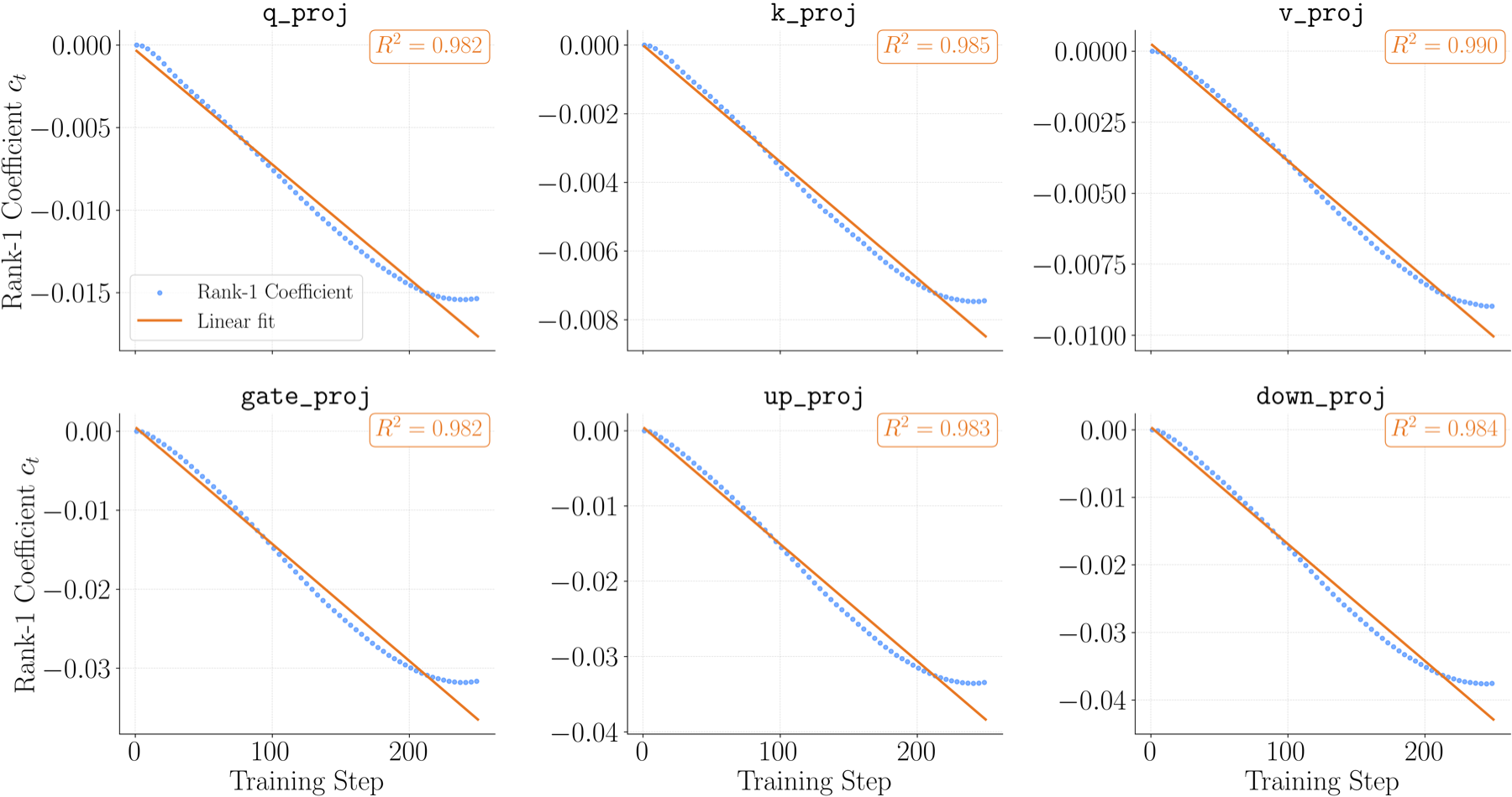
Figure 3. Rank-1 SVD coefficients evolve nearly linearly. Rank-1 coefficients (blue dots) and linear fits (pink) for representative modules of Qwen2.5-Math-1.5B.
Together, the above two findings reduce the prediction of RLVR checkpoints into a straightforward two-step process:
(1) estimate the rank-1 direction \(\mathbf{v}_1\) from the observed prefix via SVD
(2) extrapolate the scalar coefficient \(c_{T}\) of the target step \(T\) via a linear fit
Figure 4 illustrates the core intuition, and RELEX (Alg. 2) is the direct realization of it.
Method
RELEX: Linear extrapolation of SVD coefficients
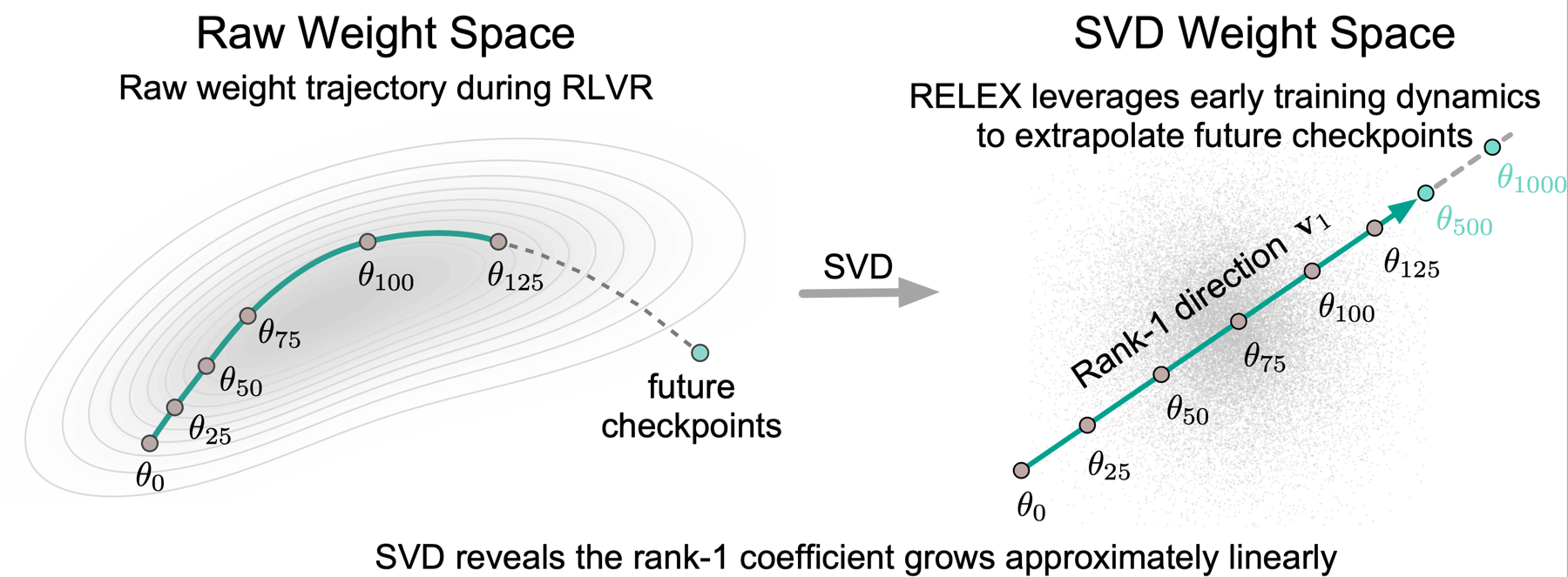
Figure 4. From raw RLVR trajectories to rank-1 extrapolation. Left: RLVR checkpoints form a curved path in raw weight space, making future checkpoints hard to predict directly. Right: after SVD, the dominant direction \(\mathbf{v}_1\) captures the main update, and the corresponding scalar coefficient grows approximately linearly with training step. RELEX uses the observed prefix \(\theta_{\le T_{cut=125}}\) to estimate \(\mathbf{v}_1\), fits this rank-1 coefficient trajectory, and extrapolates along the same direction to predict future checkpoints such as \(\theta_{500}\) or \(\theta_{1000}\) without additional RLVR training.
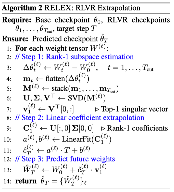
Core idea of RELEX (detailed in Alg. 2):
For each weight tensor, fit a line to its observed rank-1 coefficient trajectory \(c_t^{(\ell)}\) over the first \(T_{cut}\) steps of actual RLVR training, then extrapolate this line to predict the coefficient \(\hat{c}_T^{(\ell)}\) at a future target step \(T\).
- Observe an early prefix of RLVR checkpoints (e.g., 15–20% of the full RLVR run)
- For each weight tensor \(W^{(\ell)},\) compute deltas \(\Delta\theta_t^{(\ell)} = W_t^{(\ell)} - W_0^{(\ell)}\) and stack them across observed steps into a trajectory matrix
- Apply SVD to this trajectory matrix to obtain the rank-1 direction \(\mathbf{v}_1^{(\ell)}\) and coefficient sequence \(c_t^{(\ell)}\)
- Fit \(c_t^{(\ell)} \approx a^{(\ell)}t + b^{(\ell)}\) by least squares over the observed steps \(t_{\le T_{cut}}\)
- Predict the future coefficient \(\hat{c}_T^{(\ell)} = a^{(\ell)}T + b^{(\ell)}\) for any target step \(T_{> T_{cut}}\)
- Construct the predicted tensor as \(\hat{W}_T^{(\ell)} = W_0^{(\ell)} + \hat{c}_T^{(\ell)} v_1^{(\ell)}\), and assemble all tensors into the predicted checkpoint \(\hat{\theta}_T\)
Algorithm 2: RLVR Extrapolation with RELEX
Main Results
We train three models (i.e., Qwen2.5-Math-1.5B, Qwen3-4B-base, Qwen3-8B-base) with GRPO for 500 steps on MATH, and evaluate models on both in-domain task (MATH test set) and five out-of-domain (OOD) benchmarks.
The empirical results are surprising: using only 15–20% of the 500-step RLVR run as observed prefix, RELEX achieves comparable or even better performance than full RLVR across three models. Specifically, we use a 15% prefix for Qwen2.5-Math-1.5B and Qwen3-4B-Base, and a 20% prefix for Qwen3-8B-Base.
In-domain evaluation result: RELEX matches full RLVR performance with significantly less training cost
This shows that early RLVR dynamics contain surprisingly strong predictive signal. In many cases, a short training prefix is enough to extrapolate a checkpoint with near-final performance.
| Method (Training Cost) | Qwen2.5-Math-1.5B | Qwen3-4B-Base | Qwen3-8B-Base |
|---|---|---|---|
| Base (0%) | 48.2 | 64.0 | 73.9 |
| RLVR (100%) | 71.5 | 85.5 | 88.5 |
| RELEX (15%-20%) | 71.6 | 85.6 | 87.4 |
OOD evaluation result: RELEX generalizes well and often beats full RLVR beyond the training domain
Beyond the in-domain MATH test set, RELEX also transfers well to unseen math reasoning benchmarks. In the two smaller models, RELEX even achieves a higher OOD average than full RLVR, suggesting that extrapolation along the dominant rank-1 trajectory preserves broadly useful reasoning improvements rather than simply fitting the training distribution.
Qwen2.5-Math-1.5B
| Method (Training Cost) | AIME25 | AIME26 | HMMT25 | OlympBench | AMC23 | Average |
|---|---|---|---|---|---|---|
| Base (0%) | 4.2 | 5.0 | 0.8 | 23.2 | 33.1 | 13.3 |
| RLVR (100%) | 4.6 | 7.9 | 0.4 | 31.5 | 54.4 | 19.8 |
| RELEX (15%) | 8.8 | 10.0 | 2.1 | 31.4 | 56.2 | 21.7 |
Qwen3-4B-Base
| Method (Training Cost) | AIME25 | AIME26 | HMMT25 | OlympBench | AMC23 | Average |
|---|---|---|---|---|---|---|
| Base (0%) | 7.9 | 8.8 | 0.8 | 31.6 | 43.8 | 18.6 |
| RLVR (100%) | 23.8 | 23.8 | 10.0 | 46.6 | 64.1 | 33.7 |
| RELEX (15%) | 23.8 | 19.2 | 14.6 | 47.4 | 67.2 | 34.4 |
Qwen3-8B-Base
| Method (Training Cost) | AIME25 | AIME26 | HMMT25 | OlympBench | AMC23 | Average |
|---|---|---|---|---|---|---|
| Base (0%) | 10.0 | 7.1 | 2.9 | 36.9 | 53.8 | 22.1 |
| RLVR (100%) | 29.2 | 25.4 | 16.3 | 49.5 | 73.8 | 38.8 |
| RELEX (20%) | 27.5 | 24.6 | 15.4 | 49.6 | 72.8 | 38.0 |
Ablation and Analysis
On RELEX’s design choices: simplicity beats complexity
Beyond the impressive results of RELEX, we also provide ablations to understand why such a simple method works. Specifically, we ablate the following three design choices:
- Operating in the SVD subspace rather than the raw weight space
- Using a rank-1 projection vs. using higher ranks
- Extrapolating with a linear function vs. polynomial or neural functions
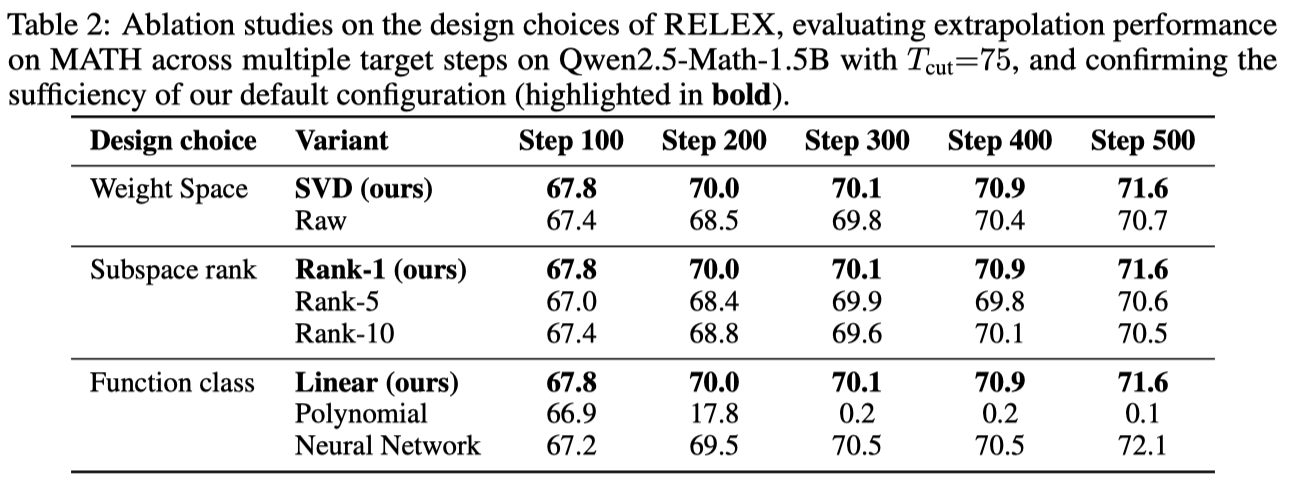
In Table 2, we ablate each on Qwen2.5-Math-1.5B with \(T_{cut}=75\).
To supplement the ablations, we further visualize the Rank-5 SVD coefficient trajectories for a representative module in Figure 5.
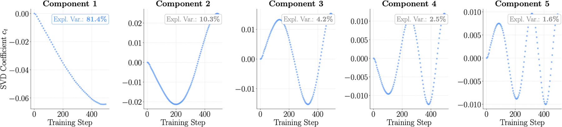
Figure 5. Rank-5 SVD coefficient trajectories for a representative tensor (layer 14 gate_proj, Qwen2.5-Math-1.5B). Annotation boxes show explained variance within the rank-5 subspace. Component 1 alone accounts for 81.4% of the variance and evolves near-linearly over training, while components 2-5 together explain only 18.6% and exhibit noisier dynamics.
Key ablation findings:
SVD projection acts as a spectral denoiser
When we extrapolate directly in raw weight space, performance consistently drops. This suggests that raw parameter updates contain noisy residual directions that are harmless inside the observed trajectory but get amplified during extrapolation. SVD helps by isolating the dominant, stable update direction and filtering out less predictable components.
Rank-1 is sufficient for extrapolation
Although rank-5 or rank-10 approximations capture more variance, they do not improve extrapolation. The reason is visible in the coefficient trajectories: the first SVD component explains most of the rank-5 variance and evolves smoothly, while components 2–5 are smaller, noisier, and less monotonic. For prediction, more components are not necessarily more useful as they can add unstable signal.
Linear extrapolation is an effective and the simplest choice, more complex predictors do not provide a reliable advantage
We compare linear regression, polynomial fitting, and a neural predictor on the rank-1 coefficient trajectory. Polynomial extrapolation collapses outside the observed window, and the neural predictor is competitive but requires careful fine-tuning. Linear extrapolation is therefore the best default: closed-form, parameter-free, and aligned with the empirical near-linearity of the rank-1 coefficient.
RELEX extrapolates stably far beyond the observed window
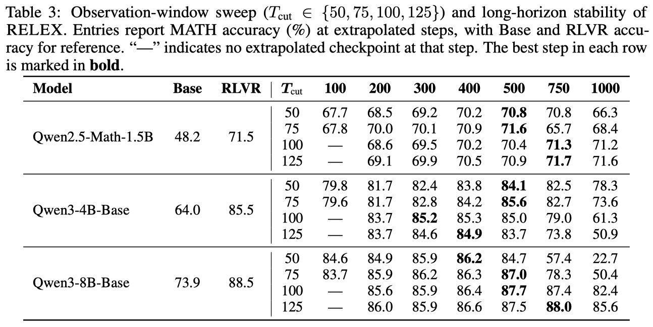
Table 3 confirms that RELEX is able to extrapolate substantially beyond the observation window, predicting checkpoints up to \(20\times\) the training steps with continued improvements (e.g., observe only the first 50 steps and extrapolate to 1000 steps), all at zero training cost.
RELEX is fairly robust across reasonable observation windows, while the long-horizon behavior seems to be model-dependent: Qwen2.5-Math-1.5B benefits from larger observed prefixes, Qwen3-4B-Base works best with a smaller early window, and Qwen3-8B-Base benefits from intermediate-to-larger windows. This makes adaptive selection of \(T_{cut}\) a meaningful direction for future extensions.
What’s Next
This work shows that RLVR training is extremely low-rank and predictable in the settings we study, but several natural questions remain:
- SFT vs. RLVR: Does the same low-rank linear structure hold for supervised fine-tuning? A systematic comparison is needed to reveal whether linearity is specific to RL’s reward-driven optimization or a general property of fine-tuning.
- RLVR tasks: We focus on math problems in this work. Does the rank-1 linearity hold for other RLVR tasks such as coding, or even tasks without verifiable rewards?
- Model families: We study Qwen2.5-Math-1.5B, Qwen3-4B-Base, and Qwen3-8B-Base in this work. Do other models (e.g., Llama, Gemma, etc.) exhibit the same geometry?
- Theoretical mechanism: Why is RLVR near-linear in SVD weight space? We conjecture it amplifies certain pre-training directions rather than learning new ones, but its theoretical support is still under-explored — exploring potential connections to neural tangent kernel theory or feature learning frameworks would be meaningful.
Citation
@article{wei2026relex,
  title   = {You Only Need Minimal RLVR Training: Extrapolating LLMs via Rank-1 Trajectories},
  author  = {Wei, Zhepei and Zhu, Xinyu and Chen, Wei-Lin and Huang, Chengsong and Huang, Jiaxin and Meng, Yu},
  journal = {arXiv preprint arXiv:2605.21468},
  year    = {2026}
}
We're excited to share these early results and welcome feedback from the community as we continue to refine the work. If you have any questions or feedback, please feel free to contact us at zhepei.wei@virginia.edu.